Reactors

canterax.ReactorNet advances constant-pressure adiabatic reactor trajectories using JAX-based ODE solvers.

Model scope

The current reactor path is:

• zero-dimensional

• constant pressure

• adiabatic

The state vector is arranged as:

[T, Y_0, Y_1, ..., Y_{n-1}]

Basic usage

import cantera as ct
import jax.numpy as jnp

from canterax import ReactorNet, Solution

gas = Solution("gri30.yaml")
gas.TPX = 1200.0, ct.one_atm, "H2:2.0, O2:1.0, N2:3.76"

net = ReactorNet(gas.mech)
sol = net.advance(
    T0=gas.T,
    P=gas.P,
    Y0=jnp.array(gas.Y),
    t_end=1e-3,
)

Solver choices

By default, advance(...) uses Diffrax Kvaerno5, which is a stiff implicit Runge-Kutta method.

You can also request the experimental custom BDF path:

sol = net.advance(
    T0=gas.T,
    P=gas.P,
    Y0=jnp.array(gas.Y),
    t_end=1e-3,
    solver="bdf",
)

Output shape

Default Diffrax path:

• sol.ts contains saved times

• sol.ys contains saved states

• sol.ys[:, 0] is temperature

• sol.ys[:, 1:] are species mass fractions

Experimental BDF path:

• returns a dictionary-like structure with ts, ys, and stats

• stats includes step and function-evaluation counters

Saving trajectories

Use Diffrax SaveAt if you want samples at prescribed times.

import diffrax
import jax.numpy as jnp

ts = jnp.linspace(0.0, 1e-3, 200)
saveat = diffrax.SaveAt(ts=ts)
sol = net.advance(
    T0=gas.T,
    P=gas.P,
    Y0=jnp.array(gas.Y),
    t_end=1e-3,
    saveat=saveat,
)

Practical notes

• Y0 should be a JAX array if you are staying in a JAX-native workflow.

• The reactor implementation is designed for differentiable simulation, but the current docs focus on forward simulation behavior.

• The BDF path is marked experimental and has more limited differentiation support than the default Diffrax solver.

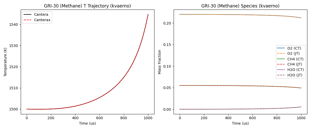
Validation image

The repository includes parity plots comparing Canterax and Cantera reactor trajectories.